Using Computer Vision to Find Lane Lines on Road
Identifying lanes on the road is a common task performed by all human drivers to ensure their vehicles are within lane constraints when driving, so as to make sure traffic is smooth and minimize chances of collisions with other cars due to lane misalignment.
Similarly, it is a critical task for an autonomous vehicle to perform. It turns out that recognizing lane markings on roads is possible using well known computer vision techniques. Some of those techniques will be covered below.
The goal of this project, the first of Term 1 of the Udacity Self Driving Car Engineer Nanodegree, is to create a pipeline that finds lane lines on the road using Python and OpenCV.
Setup
Udacity provided sample images of 960 x 540 pixels to train our pipeline against. Below are two of the provided images.

White vs Yellow Lane Lines
The Pipeline
In this part, we will cover in detail the different steps needed to create our pipeline, which will enable us to identify and classify lane lines. The pipeline itself will look as follows:
Convert original image to HSL Isolate yellow and white from HSL image Combine isolated HSL with original image Convert image to grayscale for easier manipulation Apply Gaussian Blur to smoothen edges Apply Canny Edge Detection on smoothed gray image Trace Region Of Interest and discard all other lines identified by our previous step that are outside this region Perform a Hough Transform to find lanes within our region of interest and trace them in red Separate left and right lanes Interpolate line gradients to create two smooth lines The input to each step is the output of the previous step (e.g. we apply Hough Transform to region segmented image).
Convert To Different Color Spaces
While our image is currently in RBG format, we should explore whether visualizing it in different color spaces such as HSL or HSV to see whether they can help us in better isolating the lanes. Note that HSV is often referred to as HSB (Hue Saturation and Brightness). I was trying to get my head around the major differences between these two color codes and came across this resource the other day which summed it quite well:
HSL is slightly different. Hue takes exactly the same numerical value as in HSB/HSV. However, S, which also stands for Saturation, is defined differently and requires conversion. L stands for Lightness, is not the same as Brightness/Value. Brightness is perceived as the “amount of light” which can be any color while Lightness is best understood as the amount of white. Saturation is different because in both models is scaled to fit the definition of brightness/lightness.
The diagrams below enable one to visualize the differences between the two:
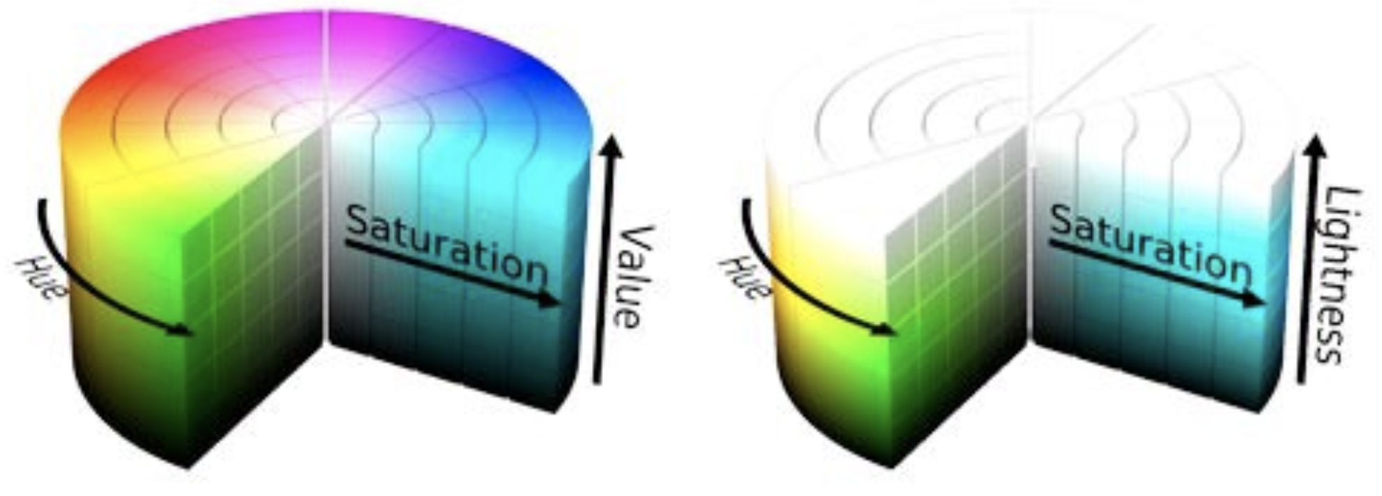
HSL and HSV color spaces
The image below shows the original image next to its HSV and HSL equivalents:
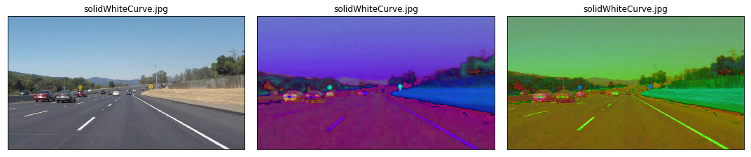
Original vs HSV vs HSL
As can be seen while comparing images, HSL is better at contrasting lane lines than HSV. HSV is “blurring” our white lines too much, so it would not be suitable for us to opt for it in this case. At the very least it will be easier for us to isolate yellow and white lanes using HSL. So let’s use it.
Isolating Yellow And White From HSL Image
We first isolate yellow and white from the original image. After doing so, we can observe how the yellow and the white of the lanes are very well isolated.
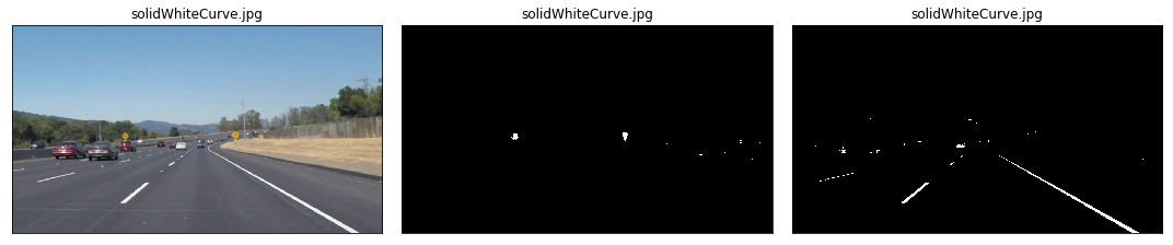
Original image vs HSL Yellow and White Line Filters
Let’s now combine those two masks using an OR operation and then combine with the original image using an AND operation to only retain the intersecting elements.
The results are very satisfying so far. See how the yellow road signs are clearly identified thanks to our HSL yellow mask! Next we move to grayscaling the image.
Convert To Grayscale
We are interested in detecting white or yellow lines on images, which show a particularly high contrast when the image is in grayscale. Remember that the road is black, so anything that is much brighter on the road will come out with a high contrast in a grayscale image.
The conversion from HSL to grayscale helps in reducing noise even further. This is also a necessary pre-processing step before we can run more powerful algorithms to isolate lines.
Combined HSL Images With Grayscale
Gaussian Blur
Gaussian blur (also referred to as Gaussian smoothing) is a pre-processing technique used to smoothen the edges of an image to reduce noise. We counter-intuitively take this step to reduce the number of lines we detect, as we only want to focus on the most significant lines (the lane ones), not those on every object. We must be careful as to not blur the images too much otherwise it will become hard to make up a line.
The OpenCV implementation of Gaussian Blur takes a integer kernel parameter which indicates the intensity of the smoothing. For our task we choose a value of 11.
The images below show what a typical Gaussian blur does to an image, the original image is on the left while the blurred one is to its right.
Grayscale (left) vs Gaussian Blur (right)
Canny Edge Detection
Now that we have sufficiently pre-processed the image, we can apply a Canny Edge Detector, whose role it is to identify edges in an image and discard all other data. The resulting image ends up being wiry, which enables us to focus on lane detection even more, since we are concerned with lines.
The OpenCV implementation requires passing in two parameters in addition to our blurred image, a low and high threshold which determines whether to include a given edge or not. A threshold captures the intensity of change of a given point (you can think of it as a gradient). Any point beyond the high threshold will be included in our resulting image, while points between the threshold values will only be included if they are next to edges beyond our high threshold. Edges that are below our low threshold are discarded. Recommended low:high threshold ratios are 1:3 or 1:2. We use values 50 and 150 respectively for low and high thresholds.
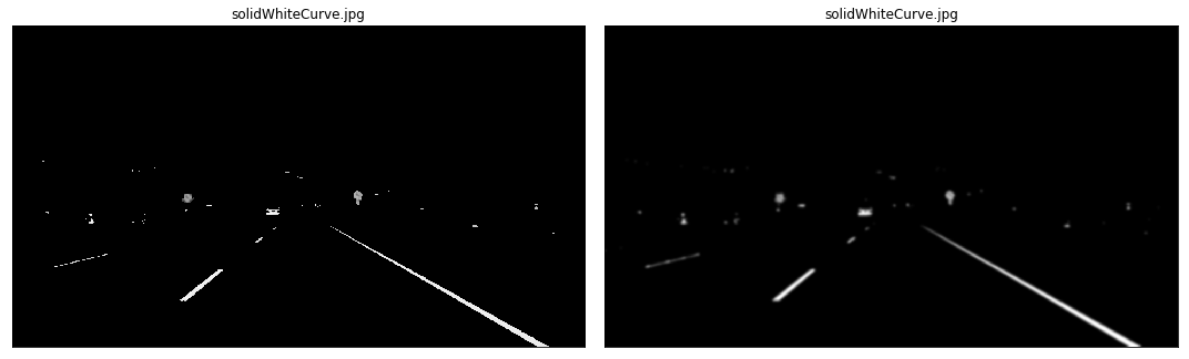
We show the smoothened grayscale and canny images together below:
Grayscale (left) vs Canny Edge (right)
Region Of Interest
Our next step is to determine a region of interest and discard any lines outside of this polygon. One crucial assumption in this task is that the camera remains in the same place across all these image, and lanes are flat, therefore we can identify the critical region we are interested in.
Looking at the above images, we “guess” what that region may be by following the contours of the lanes the car is in and define a polygon which will act as our region of interest below.
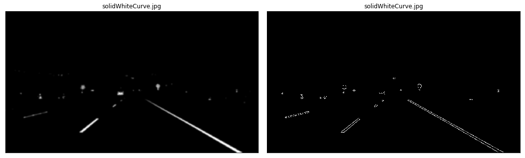
We put the canny and segmented images side by side and observe how only the most relevant details have been conserved:
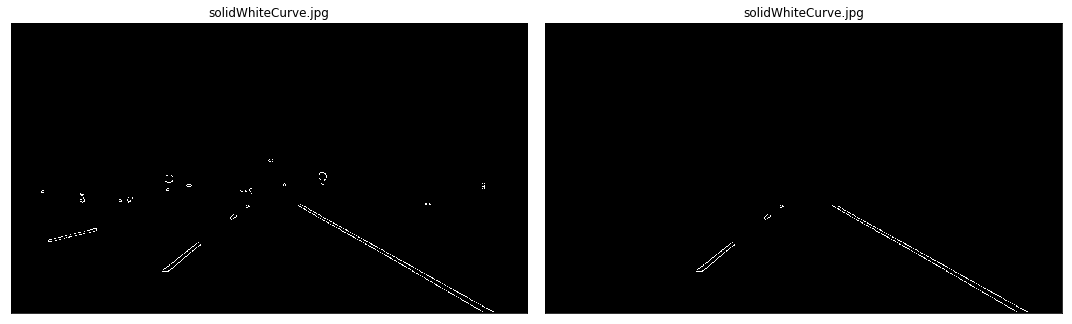
Canny Edge (left) vs Segmented Canny Edge (right)
Hough Transform
The next step is to apply the Hough Transform technique to extract lines and color them. The goal of Hough Transform is to find lines by identifying all points that lie on them. This is done by converting our current system denoted by axis (x,y) to a parametric one where axes are (m, b). In this plane:
lines are represented as points points are presented as lines (since they can be on many lines in traditional coordinate system) intersecting lines means the same point is on multiple lines Therefore, in such plane, we can more easily identify lines that go via the same point. We however need to move from the current system to a Hough Space which uses a polar coordinates system as our original expression is not differentiable when m=0 (i.e. vertical lines). In polar coordinates, a given line will now be expressed as (ρ, θ), where line L is reachable by going a distance ρ at angle θ from the origin, thus meeting the perpendicular L; that is ρ = x cos θ + y sin θ. All straight lines going through a given point will correspond to a sinusoidal curve in the (ρ, θ) plane. Therefore, a set of points on the same straight line in Cartesian space will yield sinusoids that cross at the point (ρ, θ). This naturally means that the problem of detecting points on a line in cartesian space is reduced to finding intersecting sinusoids in Hough space.
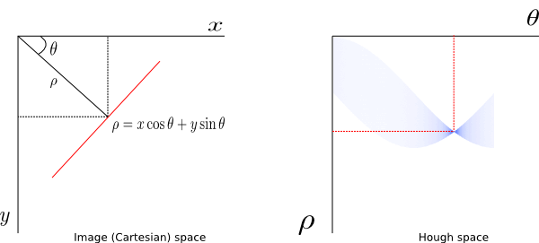
Hough Space
More information about the implementation of Hough Transform in OpenCV can be found here.
The Hough transform returns lines, and the below images show what they look like:

Hough Lane Lines Highlighted In Red
Separating Left And Right lanes
To be able to trace a full line and connect lane markings on the image, we must be able to distinguish left from right lanes. Fortunately, there is a trivial way to do so. If you carefully look the image (may be easier with the canny segmented images), you can derive the gradient (i.e slope) of any left or right lane line:
left lane: as x value (i.e. width) increases, y value (i.e. height) decreases: slope must thus be negative right lane: as x value (i.e. width) increases, y value (i.e. height) increases: slope must thus be positive We can therefore define a function that separates lines into a left and right one. We must be careful when the denominator of the gradient (the dx in dy/dx) is 0, and ignore any line with such line.
In the below images, we color identified lines belonging to the left lane in red, while those belonging to the right lane are in blue:
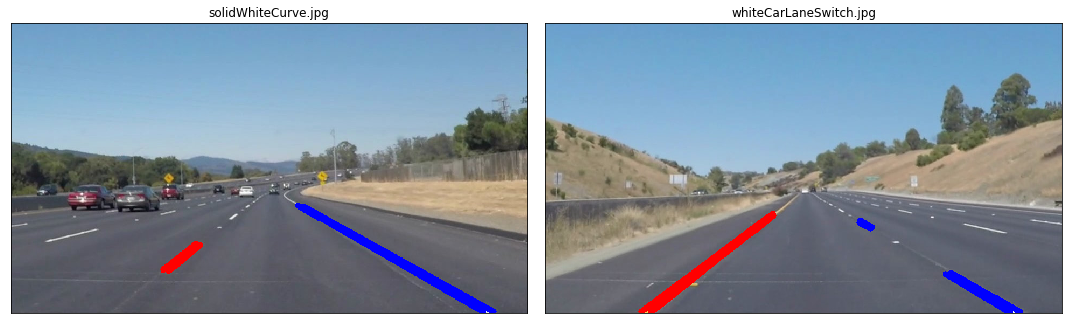
Left Lane Red, Right Lane Blue
Gradient Interpolation and Line Extrapolation
To trace a full line from the bottom of the screen to the highest point of our region of interest, we must be able to interpolate the different points returned by our Hough transform function, and find a line that minimizes the distance across those points. Basically this is a linear regression problem. We will attempt to find the line on a given lane by minimizing the least squares error. We conveniently use the scipy.stats.linregress(x, y) function to find the slope and intercept of our lane line.
We succeed in doing so, as attested by the following images below:
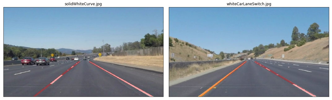
Full Lane Lines Identifiesd
Videos
Setup
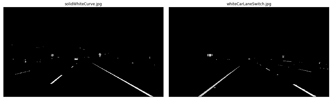
Three videos were also provided to run our pipeline against them:
a 10 seconds video with only white lane lines a 27 seconds video with a continuous yellow lane line on the left and dotted white lane line on right a challenge video where the road is slightly curved and the resolution of frames is higher
First implementation
The initial implementation worked passably on the first two videos but utterly failed on the challenge exercise. To make the line detection smoother and take advantage of the sequencing and locality of each frame (and therefore lines), I decided to interpolate lane gradients and intercepts across frames, and discard any line that deviated too much from the computed mean from previous frames.
Lane Detector With Memory Of Previous Frames
Remember that a video is a sequence of frames. We can therefore use the information from previous frames to smoothen the lines that we trace on the road and take corrective steps if at frame t our computed lines differ disproportionately from the mean of line slopes and intercepts we computed from frames [0, t-1].
We therefore need to impart the concept of memory into our pipeline. We will use a standard Python deque to store the last N (I set it at 15 for now) computed line coefficients.
This worked fairly well on the first two video and even managed to honorably detect lane lines on the challenge video, but because of the curvature of the lanes a straight line formed by a simple polynomial of degree 1 (i.e. y = Ax¹ + b) would not be enough. In the future I’ll work on better fitting lane lines on curvy roads.
The video below shows the pipeline in action on the challenge video:
Shortcomings
I have observed some problems with the current pipeline:
- in the challenge video at around second 5 the lane is covered by some shadow and my code originally failed to detect it. I managed to fix this issue by applying the HSL color filtering as another pre-processing step.
- straight lines do not work when there are curves on the road :)
- Hough Transform is tricky to get right with its parameters. I am not sure I got the best settings
Future Improvements
One further step to explore would be to calculate the weighted average of line coefficients in our MemoryLaneDetector, giving a higher weight to more recent coefficients as they belong to more recent frames; I believe frame locality would play a critical role in getting near-perfect lines on video.
We should also consider expressing lines as second degree polynomials or more for examples such as the challenge video.
In the future, I also plan to use deep learning to identify lanes and compare those results against what I obtained with a pure computer vision approach.
All code is available on Github.
This was an exciting and challenging first project that got me to understand a lot more about color spaces, image processing and revise some linear algebra too. I am looking forward to even more challenging projects that stretch my knowledge in all these fields and more, and help me in understanding how a self-driving car is built!